The first evidence for variation of gravity with latitude came when the astronomer Jean Richer took pendulum clocks with him to Cayenne and discovered that when they were that close to the equator they ran noticeably slow, even though they had kept perfect time in Paris. The effect seems not to have been anticipated, although once it had been observed, explanations quickly followed, notably from Isaac Newton. Pendulums were then used on the two French expeditions, the one to Lapland and the other to Ecuador, as supplementary methods of solving the vexed question of the gross shape of the Earth (the primary method, of course being the precise measurement of the length of a degree of latitude). For the next hundred and fifty years the study of the shape of the Earth remained the main reason for measuring gravity, and using pendulums to do so.
There were two methods. The first was what one might call ‘Richer’s method. Measurements were made of the rate of gain or loss of time by a very good pendulum clock, over periods of days. This was seen as a rather indirect way of monitoring the changes, since the escapement mechanism that provided the energy needed to keep the clock going inevitably interfered with the free oscillations, but it did have considerable advantages. There was no need for an observer to be continually and minutely monitoring the instrument, since it effectively did the counting for itself, and the observation period was long enough to remove the need for estimating fractional oscillations.
The free-swinging pendulum, on the other hand, had to be watched continually and its oscillations, steadily decreasing in amplitude, had to counted. The initial amplitudes could not be too great, or the corrections for the difference between the circle and the cycloid would become too large, but could not be too small, because there was a practical limit to how small a movement could be observed. These considerations normally restricted observations to little more than an hour, during which time a seconds pendulum (a pendulum, with a length of slightly less than a metre, with a period of exactly two seconds at the chosen reference location), would complete 1800 full periods or, to use the terminology common at the time, 3600 oscillations. This was the method used on the Malaspina expedition to measure gravity at seventeen points over a wide range of latitudes in both the northern and southern hemispheres, by observations extending over exactly one hour and oscillations countedto the nearest second. At the poles (to which he got no closer than Alaska), his pendulum would have made fewer than 3610 oscillations, so effectively, despite all the efforts of his observers, the best they could do was divide each hemisphere into ten bands corresponding to the ten whole numbers 3600 to 3609. To improve on that, with a free-swinging pendulum, a better method had to be found.
And, a few decades later, it was. Free-oscillations were used by Kater when he revolutionised the business of determining absolute gravity by the use of a reversible pendulum. For each experimental determination he observed his pendulum for only eight minutes, and he made his timings to the nearest second, and yet he achieved accuracies considerably better than one part in ten thousand. How was this possible ?
The key to Kater’s success lay in a change in experimental procedure that seems at first sight trivial. Instead of counting oscillations over a fixed period of time, the number of oscillations in a whole number of seconds were counted. The timing was done using a very accurate pendulum clock that had been adjusted against astronomical observations over periods of days to beat seconds very exactly, No measurements were needed of any of the parameters (such as length and moment of inertia) of the clock pendulum because the adjustments needed to get the timing exactly right were made empirically.
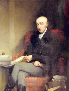
Figure 1: Portrait of William Hyde Wollaston, painted by John Jackson
I have not yet been able to discover any details of his experiments, but there is, deep in the archives of the Cambridge University Library, a collection of his notebooks and correspondence, in two boxes. Items 9 to 11 in the first box are listed as describing pendulum experiments. Presumably this is where the method of coincidences is described; it would be intriguing to know how the sound signals were generated without interfering with the motions of the pendulums, but for that a visit to the library itself is required.
On the other hand, to find out what Kater did it is only necessary to read his report. He tells us that the moment when the clock pendulum and the reversible pendulum were simultaneously at the bottom of their swing was noted, and the number of seconds then needed for this to occur again was counted. The closer the period of the reversible pendulum to the period of the clock pendulum, the longer it would take for this to happen. If it was too close, then the oscillations would be too small by the time of the next synchronisation for it to be recognised. That was one design limitation. If, on the other hand, the difference was too large, the required accuracy would not be achieved. That was the other design limitation. Effectively, instead of being measured for all possible periods, measurements were being restricted to a very small range of possible periods, which could then be examined in much greater detail. Only the clock time needed to be recorded, because the number of pendulum periods would always differ from this by exactly two seconds at the next synchronisation.
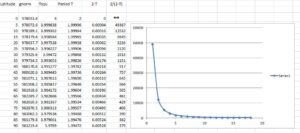 Figure 2: Wollaston’s method of coincidences
The spreadsheet in Figure 2 shows how Malaspina might have used this technique, had he known about it, with a pendulum designed to beat seconds at the equator. The first column is the latitude (north or south, it doesn’t matter which) and the second the corresponding ‘normal’ sea-level gravity, in milligals. In the third column is the square of the period of the chosen pendulum, which is directly proportional to the gravity field, and in the fourth the period itself.
The fifth column shows the differences in the periods from the standard two seconds at the equator, and the final column is the number of seconds before a second synchronisation occurs. On some occasions it was possible to record a third synchronisation, so that the count was effectively to the next half second, but this was not a necessary part of the experiment. The numbers show that even without this, instead of the entire hemisphere being divided into ten bands, each 5° of latitude would be divided into hundreds, and even thousands, of steps. This is the origin of the improved accuracy of this method, compared to mere counting of oscillations.
The graph also shows something else. Even if, as with Malaspina, the pendulum was observable for a whole hour, one would have to go to almost 20° latitude before a second synchronisation could be expected to be observable, as long as the pendulum being used was one that was designed to beat exact seconds at the equator. The obvious solution would be to use a slightly longer pendulum, and thereby ensure that even the equatorial measurements would be of a coincidence occurring only a few hundred seconds after the start. There would be some reduction in precision at higher latitudes, but the graph shows that by that stage the time to re-synchronisation would be changing only very slowly with latitude.
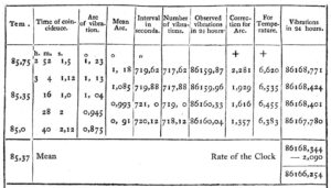
Figure 3: Results of one of John Goldingham’s pendulum experiments in Madras.
After Kater, the method was quickly and universally adopted. Figure 3 shows the results of one experimental ‘run’ made by John Goldingham in Madras a few years later. The pendulums were observed for 52 minutes, sufficient for four linked estimates. As can be seen from the final calculation, it was not even necessary for the clock to be accurate, as long as the amount by which it gained or lost time in a day was known.
Wollaston revolutionised the measurement of gravity. And he had so many other things going on, that he made little or no attempt to secure any credit for it