Having become interested in George Airy’s ‘down the mine’ Harton experiment, which I failed to describe in ‘The Hunt for Earth Gravity’, I realised with a bit of a shock that when I first began life as a geophysicist the constraints under which we worked were closer to those that Airy worked under more than a hundred years earlier than the constraints people work under today, a mere sixty years later. In 1961, armed with a degree in Physics and nothing but physics, I signed up for John Bruckshaw’s Diploma in Applied Geophysics at Imperial College. It was a course that involved force-feeding geology into physicists and physics into geologists (we had the best of that deal, I think), but memorably also it included a course in surveying which, apart from involving peering down theodolites and dumpy levels and drawing maps of valleys in Cornwall, required us to do unending calculations with log tables and mechanical calculators. When I joined Australia’s Bureau of Mineral Resources a year later, its regional gravity section (which, thankfully, I avoided) consisted of a room full of other recent graduates of about my age, all cranking away on Facit or Brunsviga machines. A year later, I was sent on a computer course in Sydney to learn how to program the University’s Silliac computer. It occupied three rooms in the Physics Building, relied on thermionic valves and must have had an instruction set of fewer than 27 instructions, because each one was represented by a single letter of the alphabet. Geophysics had, just about, entered the computer age.
But enough about me. What that preamble was for was to establish my credentials for being critical of a scientist of an earlier century. I now want to talk about George, and if I presume to be critical of a man who was Senior Wrangler of his year at Cambridge, was capable of calculating the parameters of a reference geoid that is still in use, came up with a theory of isostasy that is the basis for most modern treatments of the subject, analysed the inequalities in the motions of the Earth and Venus, was Astronomer Royal for forty-six years, etc., etc,. and who clearly had a brain with which mine could not hope to compete, I should also emphasise that I am talking about one single experiment. This is the experiment he described in his 1857 paper in the Philosophical Transactions of the Royal Society of London entitled “Account of pendulum experiments undertaken in the Harton colliery, for the purpose of determining the mean density of the Earth”. In reading this I was forewarned that Airy was notoriously a man who made great demands on his readers. In Mr Hopkins’ Men, Alex Craik noted that Airy’s seminal educational work, Mathematical Tracts, “was not an easy text for self-study; he rarely starts from first principles and takes much for granted as already know”. What seems to have been an omission in experimental practice may therefore be simply an omission in description.
The first such omission, in one or the other, is a very simple one. Airy had access to the results of attempts by Neville Maskelyne and Henry Cavendish at determining the mean density of the Earth, and at the end of his paper he compare his result with theirs. But did he, prior to the experiment, calculate the magnitude of the effect he was looking for? There is no evidence that he did, but that, surely, would have been a first step. It would have told him whether the expensive operation he was proposing was actually going to be worthwhile, and might have prompted him to look at his own results with a more jaundiced eye, to assess their variability in the light of the magnitude of the hoped-for result.
There is a second, far more certain and far more astonishing criticism. Even if Airy had calculated a rough expected result, he would not have been able to make such an assessment as the experiment progressed, because he was not there. In his account of the experiment he is explicit about the timetable. He employed six observers and stated that:
“September 30. I returned to Greenwich, leaving all in the charge of Mr. Dunkin.
October 2. Observations commenced in the morning with Swing 1”.
And later
“October 21. Observers for the day, Mr. POGSON and Mr. RUMKER, from the end of Swing 80 to the beginning of Swing 82: the end of Swing 82 was observed by Mr. DUNKIN and Mr. POGSON. The Fourth Series and the whole operation closed with Swing 82.
October 22. I arrived from Greenwich”.
So, during the whole of the operation, Airy was actually somewhere else!
This seems extraordinary. In his youth Airy had attempted a similar determination at the Dolcoath tin and copper mine in Cornwall, and his failure there must have been niggling at him ever since, because when a solution emerged to one of his greatest problems, the problem of sending signals instantaneously between the observer down the mine and the observer on the surface, he decided to try again. By 1854 he could do that by simply completing an electrical circuit to cause a galvanometer needle to kick over. After waiting 30 years, one would have thought he would want to see the whole operation up and running for at least one day before he set off back to London. Instead, he left it in charge of Edwin Dunkin, who was one of his assistants at the Royal Observatory, and that may have been a mistake. Not because Dunkin was incompetent, but because in the first week he was seized with a sudden and severe illness (p. 331). Airy noted that this delayed the sending of the observations (presumably in part via the newly opened Great Northern Railway), but it must surely also have has some effect on the operations.
The use Airy made of electrical signals was also curiously limited. It was based on a single circuit that could be broken at three points. Two of these were controlled by the two observers, and were normally closed, the third was controlled by a ‘journeyman clock’, i.e. a clock of which extreme accuracy was not required, because all it had to do was make the circuit every fifteen seconds. The only way one observer could communicate with the other was to break the circuit and then rely on the other observer to note that the expected 15-second galvanometer kick had not occurred. Anything approaching a conversation between the two had to rely on a necessarily small number of pre-arranged signals involving stoppages in different patterns, extending over multiple 15-second intervals. One can think of many elaborations to this very basic scheme that would have improved things, the simplest being a switch that allowed the upper observer to bypass the circuit-breaker in the clock and send quite complex instructions to his underground colleague.
Nothing of that sort seems to have been done. Airy simply installed the ‘Shelton’ clock (conveniently, ‘S’ for surface) and the journeyman clock in the upper observatory, the ‘Earnshaw’ clock in the observatory underground and the signal wires running between the two, all with great care and attention to detail. The observations could then be begun. The clocks were of the highest possible quality and both beat approximate seconds, but since neither had been calibrated against astronomical time, the observations of the difference between the two are most easily considered by regarding the ‘Shelton seconds’ as the standard. The comparison of the rates of the two clocks was done in parallel with the observations of the periods of swing of the ‘detached’ pendulums that were used to measure relative gravity. Necessarily it was done with the clocks in their experimental positions because ‘Earnshaw’, the pendulum clock used underground, would be affected by the change in gravity going that Airy wished to measure.
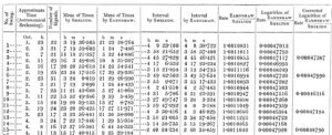
Figure 1. The beginning of Airy’s tabulation of the comparison of the two clocks. Comparisons were made after each ‘swing’. The ‘number of signals’ column records the number of times a signal was received from the journeyman clock. Although this clock was not accurately calibrated, these numbers were taken as being sufficient to estimate the number of coincidences during each swing. One useful aspect of this table is that working through the intermediate steps confirmed the supposition that Airy’s logarithms were to the base 10.
In presenting his results, Airy relied on tabulations of the sort shown in Figure 1, which end, inevitably, in two columns of logarithmic values. Airy, of course, was a great mathematician, and could presumably look at such a tabulation and make instant sense of it. We lesser mortals (or me at least) prefer something more visual, and in Figure 2 the full results are presented in graphical form, with the calculations taken a little bit further to show the beating of the ‘Earnshaw’ clock in Shelton seconds per Shelton day, i.e. the number of Earnshaw beats to 86,400 Shelton beats.
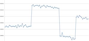
Figure 2. Plot of the results of the comparison of the two clocks.
Figure 2 raises all sorts of questions. Firstly, although Airy is adamant that ‘Shelton’ remained on the surface and ‘Earnshaw’ was always underground, it is clear that something was done to the clocks when the detached pendulums were interchanged. Airy admitted as much on p. 311 when he wrote that “It will be remarked that the pendulums of the clocks were altered at the times of interchanging the detached pendulums; that is, between Swings 26 and 27, between 52 and 53, and between 67 and 68” but, frustratingly, gave no indication of what was done or why. It would, one feels, have been much better to have left those clocks completely undisturbed, and there is some justification for this attitude in the graph itself; there is no long-term trend in the comparison during the first series of swings, but such trends are obvious during subsequent swings, and cast some doubt on the validity of the results from those swings. If they had been either longer or shorter, the averages used in the subsequent calculations would have been different. If the clocks had not been interfered with, the lackof a long-term increase or decrease might have continued.
A further question raised concerning the accuracy. At first sight it looks impressive, with variations of only a few seconds in 86,400 seconds, but this becomes less impressive when considered in the context of the accuracy required. At the end of it all, Airy concluded that “The acceleration of a seconds’ pendulum below is 2.24 per day, with an uncertainty of less than O.001” (p. 330). Those 2.24 seconds were, of course, the total effect he was looking for, and to improve on Cavendish he needed an estimate correct to the second decimal place. The standard deviation of the Series 1 rates, however, is about 1.1 seconds, or almost half the difference to be measured, and the values around the mean lines in the subsequent swings would be little different. On these grounds alone, a 20% error in the final results would be disappointing but not astonishing.
This possible contribution to Airy’s error concerns only the clocks; the estimating of the periods of the detached pendulums has not yet even been introduced, and the first necessity there is an understanding of the method of coincidences. Early users of pendulums such as Alejandro Malaspina simply counted the number of swings, to the nearest whole swing, in a known number of seconds. If Airy had used the method, with observation periods of generally something over 10,000 seconds, he would have had little hope of determining the periods to anything approaching one second, let alone the 0.01 second he claimed. To achieve this he relied on thean ingenious method first suggested by William Wollaston and routinely used thereafter by people such as Henry Kater and Edward Sabine. In this method the time taken for a detached pendulum to gain or lose one whole period (two swings) against the pendulum of a well-calibrated pendulum clock beating seconds was measured, usually to the nearest second.
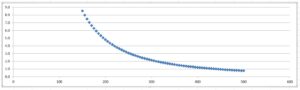
Figure 3. Plot of the effect of one unit changes in the function n/(n-2) with n varying from 150 to 500.
The method relies for its increased precision on the very non-linear nature of the relationship between the numbers n and n-2. For the longest of Airy’s observed swing intervals, of almost 500 seconds, a one second error in the estimate of a coincidence interval produces an error of less than a second in the daily rate, but this is still large in terms of the total change of 2.24 seconds between the two stations. For the shortest swing, of about 300 seconds, the situation is considerably worse, with a one second error leading to a 2 second error in daily rate. Admittedly, Airy could argue that the multiple interval values that he averaged into a single value for each swing allowed him to quote periods to a fraction of a second and also reduce the noise level. We do not know that those noise levels, or variability within a single swing, were, but If the errors could be assumed to be random, then the 26 swings of the first series would be expected to produce a five-fold noise-level reduction. Against that, however is the fact that the errors, however great or small they might be, would occur with both pendulums, swinging simultaneously.
Figure 4. Tabulation of the results of the comparison of the two pendulums, which were interchanged after each series. Vertical scale is ‘rate’, in oscillations per day. The ‘log rates’ in the final column are obtained by adding 10 to the log of the rate of the detached pendulum on the Shelton clock, but it is not clear why Airy did this, rather than use the actual logarithm of that rate.
But were these errors random? To investigate that, Airy’s results, in seconds per day, for each of the four series of observations can be plotted.
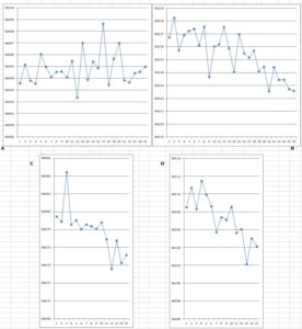
Figure 5. Plot of the results of the comparison of the two pendulums, which were interchanged after each series. Vertical scale is ‘rate’, in oscillations per day
What is very obvious is that these graphs follow the deviations due to the clock rates. Airy noted this, and stated that “On tracing the irregularities in these numbers to their sources it can be seen that they arise almost entirely from the irregularities in the comparisons of the clocks” (p. 324). As a brilliant mathematician, at home with numbers and logarithms, it is possible that he looked only at these, but his use of the word ‘tracing’ suggests that he might also have drawn the graphs. Looking at these, it is evident that the errors for the first series can be considered random, although a slight upward trend is possibly present. The standard deviation is 1.3 seconds, which again is about half of the entire difference between the two stations. For the other three series, the downward trend seen in the clock results is apparent. Airy noticed this, stating, on p. 324, that “The rate of each pendulum upon its clocks either so constant or changes by such uniform degrees in the same direction that there is every reason to presume on the extreme steadiness both of the detached pendulums and the clocks” (my underlining). But having noticed this, he appears not to have thought that it mattered. Indeed, in applying weightings to his results to allow for the assumed reliability of the different series, he gave the highest weighting to Series 2, on which the downward trend is most pronounced. Had the observations in that series been terminated after fifteen swings, as they were for Series 3 and 4, his estimate would have been very different, because in fact the downward trend seems to steepen from that point onwards.
One thing that comparison of Figures 2 and 3 does tell us is that the tortuous corrections that Airy made for temperature and air density were, in the end, almost pointless. He would have done better to focus on the clocks and see what might be done to improve things there, but it was probably hopeless. Fifty years later the Prussian Geodetic Institute went to enormous pains to measure the Earth’s gravity field at their observatory in Potsdam, using no fewer than five different pendulums, and they still got the answer wrong, by about 16 parts per million. Airy never really had much of a chance of improving on Cavendish’s determination, but fortunately for him, he never learned how inaccurate his own result had been.