A few weeks ago, David Moore of Xcalibur Multiphysics posted this on LinkedIn.
Following successful Falcon Airborne Gravity Gradiometry (AGG) surveys in Victoria during 2021, Xcalibur Multiphysics are set to begin Falcon AGG acquisition in the Cobar area of NSW from January 2022.
Looking at the success of small scale, high resolution ground gravity data in the Cobar region and the correlation of gravity highs with known mineralisation at Hera, Federation and others, we expect the regional scale, high resolution FALCON gravity gradient surveys to provide a step-change in the geological understanding of the region and hopefully allow direct targeting of new and untested mineralised systems and structure.
It was a post that took me back in my mind almost 60 years, to early 1963 and my very first survey with Australia’s Bureau of Mineral Resources, the BMR. For the organisation, and for Australia, it was also a first – the first airborne proton magnetometer survey in the country, using the instrument designed and largely built by John Newman.
This was an advance in many ways. Previous BMR aeromagnetic surveys had been carried out using fluxgate magnetometers mounted in the tail booms of the two DC3s, registrations VH-MIN and VH-BUR, and those aircraft continued to be the work-horses for the long distance coverage of the 4-mile to the inch (now 1:250,000) sheet areas. Proton magnetometer surveys were to be different, exploiting the advantages of this new instrument. First, it was not sensitive to orientation, so it could be put in a ‘bird’ trailed behind the aircraft. That removed the need for the complicated devices needed to compensate for the magnetic field of the aircraft. Also, it did not drift, so the process of turning measurements into maps would be simpler. And because the electronics were basically simpler also, it could all go in a much smaller aircraft. VH-GEO
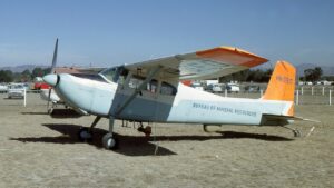
Figure 1. Cessna 180 Skywagon VH-GEO, with the ‘bird’ mounted in a cradle under the fuselage. The bulge under the fuselage further back is the aerial for the radio altimeter. GEO had an eventful few years with the BMR but was sold in 1968 and was then written off in a ground-loop at Archerfield in October 1969. Photo from the Ben Danecker collection displayed on the Air History website
In order to test the new instrument as a piece of field equipment, a place was needed which was reasonably benign from the point of view of low-level survey, where the geology was reasonably well known and where there was as much existing magnetic data as possible. That place was Cobar, where Cobar Mines Pyt Ltd was developing (or rather, re-developing) the CSA mine.
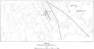
Figure 2. Geology of the one of the several test areas flown. This one is immediately south of Cobar township. The area covered is identical with the areas shown in Figures 3, 4 and 5. Figure reproduced from BMR Record 1964/110.
Other things didn’t change. Navigation was still along lines plotted on photomosaics, and because this new tool was to be used for detailed surveys at low level, the topography seemed to come at the navigator much faster than it had in the DC-3s. Lines were short, and quite soon the idea of trying to navigate while on line was abandoned altogether. The role of the ‘navigator’ was limited to trying to ensure that at least the plane was where it should be at the start of the line. He had, in any case, other things to worry about, because he was also the operator. He had to annotate the chart, which involved some contortions since the recorder was behind him (no room in front, even though the dual controls had been taken out to make a little more space) and ensure that the ink was running freely and a record was actually being obtained. Annotation was complicated, because not only did the numbers on the navigation ‘fiducial’ counter have to be written on periodically, but also, and rather more often, the magnetic field values. Readings were obtained at two-second intervals, so instead of the continuous trace provided by the fluxgate, the chart showed what was essentially a histogram; the full-scale deflection was 100 nT, and if in two seconds the field changed by a few tens of nT, there was some uncertainty as to which hundred range it was in (not a great problem in Cobar, but to become a real problem in some later surveys). Also, the operator had to install the camera and let loose the ‘bird’ at the start of each survey, and then wind in the bird and lift the camera out of its well when the last line had been flown. All this while holding down his breakfast, and at 250 ft above ground level and a survey spec that required the pilot to at least attempt to follow the terrain, things could become uncomfortable. All three of the geophysicists, and the electronics technician who kept the instruments running, had to take their turn. Only the draughtsman was exempt from airborne duties. At the start of the survey he did most of the work of ‘recovering’ the actual path taken by the aircraft from the photos, but as the results came rolling in, his job was to turn them into beautiful maps, and everyone else had to take their turn with the strip film.
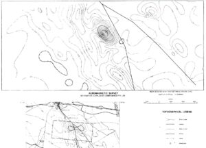
Figure 3. Results of Cobar Mines Pty Ltd semi-detailed aeromagnetic survey. Nominal flying height 300 ft a.g.l., nominal flight line spacing 0.25 mile. Inset shows the survey area positioned on the regional magnetic map from fluxgate magnetometer mounted in the BMR’s DC-3, VH-BUR. Figure reproduced from BMR Record 1964/110.
There were some differences from DC-3 practice that produced the inset map in Figure 3. There was still a downward-pointing camera, but the continuous-strip image no longer worked at low level, because it showed far too little of the ground. Instead, the camera had a ‘fish-eye’ lens with a slightly more than 180° field of view (you could see aircraft wheels at the edge of every frame) and each frame showed a circular image of the ground below, highly distorted towards the edges. Every day the camera had to be retrieved from the aircraft so the film could be removed and replaced, and then be developed and hung up to dry. Inevitably, film processing, done at the dead of night, was the job of the most junior geophysicist. Replacing the camera had to wait until the aircraft as in the air, because of the risk of damage from flying pebbles if it was in position during take-off and landing. Cobar was, of course, a dirt strip.
With the film developed and the flight path plotted, it was the turn of the magnetic data. At the beginning and end of each flight, a standard line was flown, and we assumed that the changes in the Earth’s field had been linear in that time. We had what we called a ‘storm-warning’ fluxgate magnetometer in a tent at the airstrip to tell us if that was true, but that was about all it did.***
With the baselines flown and a ‘good’ storm warning record in hand, plus a flight-line plot, mapping could begin, and that was the easy bit. Draw an estimated base line on the chart of each flight line, and draw lines parallel to it, spaced at the contour interval. Plot the contour cuts on the map, draw the contours, hand them to the draughtsman to make beautiful, And when he had done that, try one’s hand at a little first-pass interpretation.
How successful was it all? Well, we had geology and the results of the BMR’s DC3 survey, and also, in some of the areas, the ground survey (Figure 3) and the detailed airborne fluxgate survey (Figure 4) carried out by Cobar Mines for comparison, so I leave that to others to judge.
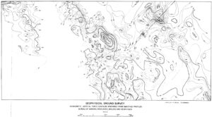
Figure 4. Results of Cobar Mines Pty Ltd ground magnetic survey. Some of the areas left blank but were not contoured because ‘noise’ from near-surface sources, both natural and artificial, made that impossible. Figure reproduced from BMR Record 1964/110.
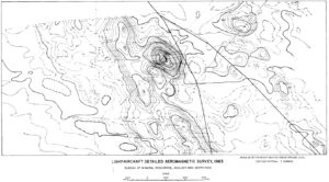
Figure 4. Results of VH-GEO detailed aeromagnetic survey. Note the ‘ticks’ on the contour lines showing the locations of flight lines. One of the advantages, compared to ground survey, was that the near-surface noise was effectively filtered out by flying at 250 ft above ground level. Figure reproduced from BMR Record 1964/110.
This much I do know. Few people starting out in airborne geophysics can have ever had a better introduction to the basics of their trade. By the time it was all over I had planned flights and marked the lines on to photomosaics, installed charts in the chart recorder and film in the camera, navigated from the seat next to the pilot while annotating the chart, extracted the chart and film, developed the film, recovered the flight path, generated the contour cuts, plotted them out and drawn the contour map. And then done a first-pass interpretation. There was not much in the airborne geophysics of the time I had not done, and the following year I went with VH-GEO to the west coast of Tasmania, Renison Bell and Tennant Creek as party chief. Fifty years later I was still applying bits of what I learnt then, to surveys that had become fully digital and had added the exotica of gravity gradiometry to the airborne package.
Thank you, BMR.
*** POSTSCRIPT. The Storm Warning Magnetometer was too sensitive to temperature change to be used to correct the airborne results, but did provide a very interesting introduction to the fact that there was more going on out in the Australian bush than airborne geophysics. Throughout our stay in Cobar, the area around the tent was the scene of an extended battle between the little ants (only about 1 – 2mm long but a lot of them) and the big ants (up to a couple of cm long, but not so many of them). The BAs were clearly the aggressors. They came charging into the LA area spreading death wherever they went, but eventually became clogged down with bodies and disappeared under a squirming pile of their dying enemies. Even so, they were winning until just before we left, when hordes of SAs appeared out of new nest areas on their flank and wiped them out.