Old men get grumpy. Things are not as they were when they were boys. For myself, my life seems to have been divided into two parts, the first with bureaucracy decreasing ever increasing , the second with it ever increasing. AsI was growing up, I.D. cards disappeared, and then ration books. Frontiers became less daunting and visas less necessary. The walls and barbed wire entanglements across Europe disappeared. Now they are going back up, and the bureaucrats are flourishing. In the UK, ‘Take back Control’ has become ‘Get used to being controlled’. Paperwork is piled on paperwork. As a school governor, I see young, enthusiastic teaches drowning in the stuff, and leaving the profession. In my own profession, accreditation now depends, not on competence but on reporting that sufficient books have been read, or enough meetings attended.
And, heaven help us, there is ASTM D5777-18 telling us how to do seismic refraction surveys.
Is that not a good thing? Should there not be standards?
In theory, the answer is an obvious yes, but look closer. A written standard too soon can become outdated, and even at its origin it is always a minimum. It is a lowest common denominator, below which one should not fall. All too easily, that becomes the benchmark of acceptability. What does ASTM D5777-18 tell us? It tells us that in doing a seismic refraction survey we should have a source to create seismic waves, and geophones to detect them, and seismographs to record the information. Did we need an anonymous committee to tell us that?
What else do they tell us? That “the interpretation formulas are based on the following assumptions: (1) the boundaries between layers are planes that are either horizontal or dipping at a constant angle, (2) there is no land-surface relief, (3) each layer is homogeneous and isotropic, (4) the seismic velocity of the layers increases with depth, and (5) intermediate layers must be of sufficient velocity contrast, thickness and lateral extent to be detected.” They imply, thereby, that if these conditions do not apply, we are helpless.
We are not.
A brief diversion
A beach, on a medium-sized island, three degrees south of the equator. A geophysicist crouches for 30 seconds over a LaCoste gravity meter, writes down some numbers in a notebook, stands up.
New to gravity survey, two watching geologists think it hilarious.
“You came all this way, just to do that?”
“I am not” says the geophysicist, “here to make this measurement.”
” I am here to decide where to make the next one.”
The right answer. In his mind is a map of the island (Buru), with the gravity contours so far. Another data point, a slightly better understanding of where the work should be concentrated in the limited time available,. That, in the essence, is why geophysicists need to go into the field. No field area should be left if there is something important that could have been done, that has not been done. For work that is rather more complicated than regional gravity, there are program packages that can be used to make early appraisal more effective. But, as they get smarter and smarter, there is a risk that we will lose ability to look at a result and think “that’s rubbish”. Or, worse still, that we will do what the packages tell us to do, rather than what needs to be done.
Refraction again
Nowhere is this more true than with shallow refraction.
Let us do what ASTM D5777-18, tells us, and fire a single shot into a spread of 12 geophones. With the first-breaks identified, the time-distance (T-D) plot might look like this:
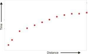
Figure 1. Plot of the ‘picks’ of the first arrivals from a ‘short-shot’ fired into a 12-geophone spread. Geophone 1, which for all other shots will be placed where this shot was fired, has been moved half-way towards the Geophone 2 location, to provide more information on the direct wave. A plot of this sort could have been generated from something as simple as an Excel spreadsheet with just two columns, the distances D of the geophones from the shot and the times of the picks.
Figure 1 looks like the plot of a 3-layer case, and indeed, the best-fit lines are easily drawn. Intercept times can be measured for the two refractors, and velocities can be estimated.
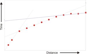
Figure 2. The same information as in Figure 1, with best-fit lines added by eye. The ‘intercept times’ are the times at which these lines cut the time-axis, and the cross-over distances are the distances from the shot point at which these lines cross each other. Drawing these lines on a single plot is not something that can be done easily within Excel, but is not a necessary step either. In fact, as what follows shows, it can even be misleading.
But, and what ASTM D5777-18, while talking in terms of the depth of the refractors below the shot point, neglects to make clear, is that at that point there is no information from the refractors. There is no way of knowing whether that apparent second cross-over is real, or the result of a change in refractor dip.
How to check? Place Geophone 1 back at what was the SP, go back a suitable distance along the extension to the line, and make a new SP. How suitable is suitable? At least as far as the suspect cross-over is from the original SP. The T-D plot could possibly then look like this.
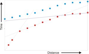
Figure 3. The short-shot data with the long shot data added, immediately raising doubts about the location of the cross-over between the two sets of refracted arrivals. Again, not something that can be done easily within Excel, but there are many packages availably that can plot points from X-Y text files with different symbols. I like using Global Mapper, because I have it to hand and because it gives me a choice of symbols for things such as schools, hospitals and golf-courses to distinguish between arrivals from different shots.
This has changed everything. The long-shot data has a kink on the same place as the assumed cross-over in the short-shot data. That suggests varying dip and possibly even a two-layer case.
To check that out, we can see whether the difference between the two sets of arrival times is constant, all the way back to the first cross over.
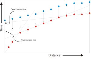 Figure 4. Confirmation that the cross-over was in the wrong place. The differences in the arrival times from the two shots only begin to vary significantly about half-way back along the spread from Geophone 12. In this figure that is being established graphically, but if the two sets of data are entered into a spreadsheet (where else are they going to be put?), the differences can be displayed numerically with a single sweep of the mouse.
So, this one is, in fact, a three-layer case, but not the one it seemed to be at first. The constant time-difference at the last six geophones can be used to ‘ghost in’ a much more reliable intercept time, because now we do have information from the vicinity of the shot point that has come up from that deeper refractor.
However, to get a depth a velocity is needed, and that information is contained in the slopes of the arrival-time plots. For Refractor 2 there seem to be choices to be made. The slope before G9, or the slope after it? Or an average of the two?
Don’t choose any of these, That will not work. Instead, shoot a long-shot from beyond the other end.
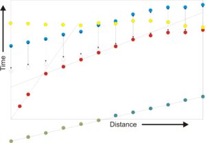
Figure 5. The data for the long-shot from beyond Geophone 12 have been added (yellow circles), and also (green circles) the differences between the arrival times from the two long-shots (once again, obtainable from the spread sheet with a single sweep of the mouse). The data from the shot to be fired at the Geophone12 position (after the geophone itself has been moved) is yet to come, but what has to be done where that is concerned should be obvious.
If the differences in the long-shot arrival times are plotted, and the line they define is roughly straight (as in Figure 5), its slope (distance divided by time) equals half the velocity along Refractor 2.
If there are some odd points that don’t fit to the line, then the ‘picks’ involved need to be looked at again. And if the line is not straight, then either the dips are extreme or the refractor velocity changes along the line. For field interpretation, it is enough to know that. The man back in the comfortable office can investigate that further
The road to hell is paved with the attractions of a drink at the bar, after a long hot day in the field, but the most time consuming part of the whole process is the picking of the arrival times and entering them into the spreadsheet. If even that is not going to be done in the field, then the field operations truly can be left to robots.