Santa Marta and WGM2012
The year 1996 saw the first serious attempt at mapping global gravity, when EGM96 was launched on the waiting world. It was understandably not a very good attempt, because of the state of the world’s gravity coverage at the time. The distribution of conventional land gravity data was very uneven, the inversion of sea-level data derived from satellite radar measurements was still in its infancy, and what gravity data was available from space came from observing perturbations in the orbits of satellites for which gravity measurement was very far from being a primary objective.
All this changed with the launch of the CHAMP satellite in 2000 and the GRACE satellites in 2002, and in 2008 a new Earth model, EGM2008, was published by the US National Geospatial Intelligence Agency (NGA). The free-air gravity grid, with 5_arc-minute cell size, was placed in the public domain on the NGA web site, but in a rather user-hostile form, having been generated on a SUN computer using a Big Endian binary format and being readable only by a special (although downloadable) Fortran program. How many users these days, I wonder, have computers that can routinely run Fortran or know enough of the jargon of machine-code programming to understand what Big Endian means. And, even if those hurdles are successfully jumped, only free-air gravity is available. One thing that is easily available, however, is the listing of the grid statistics, and this shows a global minimum value of -385.5 mGal and an astonishing maximum of +966.3 mGal.
With no geographic coordinates attached to those values, it might have been difficult to find out where they occur, but at this point the Bureau Gravimetrique International (BGI) came riding to the rescue. Not only can the EGM2008 free-air grid and a Bouguer grid derived from it be download from its website as ASCII files but also the BGI’s own WGM2012 free-air, Bouguer and isostatic grids, which are based on EGM2008. The data have to be downloaded in 100°x100° slabs, but it still doesn’t take long to discover that the very high free-air values do not occur somewhere in the Himalayas, as might be expected given the very strong dependency of free-air gravity on elevation, but in the very, very odd Sierra Nevada de Santa Marta in the extreme north-east of Colombia, which peaks at about 5700 metres.
In my blog of 31 January 2020 I started what is intended to be a series of posts about extreme gravity. This first effort looked at where on the Earth’s surface the absolute gravity field is likely to be either strongest or weakest. In that ‘competition’ the effect on gravity of the change in Earth’s radius with latitude is of paramount importance, but this is removed in the first two stages of gravity reductions, when free air gravity is calculated. The free air correction allows for the effect of elevation of the point of observation but retains the effects of all the distributed masses, whether topographic, geological or in the form of isostatic compensation. It is the isostatic compensation, the presence of a deep crustal root beneath the Himalayas, that reduces the maximum free-air gravity in the Himalayan region to a mere +630 mGal, considerably less than the Santa Marta high but still greater than in any other geographical region.
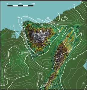
The Sierra Nevada de Santa Marta. Bouguer gravity after Kellogg and Bonini (1982)
What then of Santa Marta? It really is a very odd mountain range. It is quite small, triangular in shape, and rises straight up from the Caribbean coast of Colombia. To the south-east there is a broad valley, and then there is another small but high mountain range, this time a linear one, the Sierra de Perija along the Venezuela border. There free-air gravity is much lower, but still greater in places than anywhere in the Himalayas. What on Earth is going on? Can these values actually be believed?
In 1982 Kellogg and Bonini presented a Bouguer gravity map of NE Colombia, based on existing conventional gravity data. The main economic interest in the area is centered on exploration for hydrocarbons in the Lower Magdalena Valley SW of the Sierra Nevada and, as the map implies, there are not enough gravity stations in the Sierra itself to allow contours to be drawn. There is no doubt that the Bouguer maximum will be very high, but the lack of control only allows guesses to be made as to how high it will be.
The people who compiled EGM2008 had more strings to their bow, because they had the data from the CHAMP and GRACE satellite missions. Neither relied on simple orbital perturbation to estimate gravity. CHAMP had an on-board gravity sensor and GRACE deployed two satellites that orbited the Earth 220 km apart, allowing gravity gradients to be directly measured in space for the first time. The combination of satellite and surface gravity measurements was no small task, but it was successfully accomplished. EGM2008 was produced and from it WGM2012 was developed. However, when the WGM2012 grid is plotted for the Santa Marta, the result is very strange indeed.
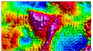
Image of the WGM2012 free-air gravity grid for the Sierra Nevada de Santa Marta. Shaded relief presentation produced in Geosoft
It is clear that something odd is happening here. Having started by wondering whether we could believe in the extraordinarily high values over the two mountain blocks, we now find ourselves faced with the near-impossibility of believing that some very strange curvilinear features are real. They look like processing artefacts and, fortunately, there is a way of checking. Offshore, EGM2008 is based on values derived from satellite altimetry, and for those we can go right back to the source, the independently published Sandwell grids.
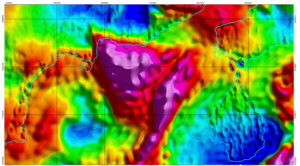
Image of the Sandwell free-air gravity grid for the Sierra Nevada de Santa Marta. Shaded relief presentation produced in Geosoft
The Sandwell free-air map is very similar to the WGM (as it should be onshore, where the Sandwell free-air grids rely on EGM2008), but the curvilinear features are absent in the areas where the Sandwell grids use the altimetric data directly. The patterns in the Caribbean show nothing remarkable and Lake Maracaibo is dominated by uncurved linears that trend a little west of north. The curvilinears are, however, present where the grid relies on non-altimetric data. There can be little doubt that the curvilinears are processing artefacts, but there is one more check to be made. Both maps were produced by contouring the grids using Geosoft routines. Could it be Geosoft that is doing this?
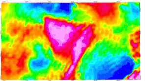
Dot-matrix image of the WGM2012 free-air gravity grid for the Sierra Nevada de Santa Marta. Zone coloured plot roduced in Geosoft
Fortunately, Geosoft does not only contour data, it can plot data using symbols that can be colour-coded for magnitude. If you use square symbols and pick the right size, a coloured map can be produced that represents the raw grid. The map is not nearly as pretty as the shaded-relief version, but one thing is clear. The curvilinears are still there. There is something odd going on with WGM2012 and possible also (depending on the source of the onshore data for the Sandwell grids), EGM2008.
I don’t pretend to understand at the moment what it is. The wave patterns look very much like those that would be generated by a sinc function, the Fourier transform of a boxcar filter. Some sort of filter would have been needed to transform the spherical harmonic system of EGM2008 to the lat/long grid of WGM2012, but perhaps the problem goes all the way back to EGM2008. And very probably it is the extreme nature of the free-air gradients in this region and the almost point-source character of the Santa Marta anomaly that make the patterns so strong. Further than that I wouldn’t want to go. But if I find out anything more, I will let you know.